Visualizing CFD Simulations: A Quick Guide to Plotting Residuals with GNUplot in OpenFOAM

Introduction

In the intricate world of Computational Fluid Dynamics (CFD), the ability to visualize and interpret simulation results is paramount. OpenFOAM, a widely recognized open-source CFD software, empowers engineers and scientists to simulate complex fluid flows, while GNUplot, a versatile data visualization tool, turns numerical data into insightful plots. Together, they form a powerful duo, enabling users to navigate through the numerical sea of simulation data, and extract meaningful visual representations. This post will whisk you through a succinct guide on extracting residuals from OpenFOAM simulations and crafting informative plots using GNUplot, in both terminal and graphical user interface (GUI) environments, paving the way for enhanced data analysis and decision-making in your CFD endeavors.

---

Extracting Residuals and Plotting with GNUplot

Navigating through the numerical data generated by CFD simulations can be a meticulous task. In an environment powered by Ubuntu 22, utilizing OpenFOAM version 10 and GNUplot 5.4.9, we can streamline this process by extracting residuals and visualizing them effectively. Let’s delve into a step-by-step guide:

A. Extracting Residual Data

Firstly, we need to extract the residual data from the log file generated by the OpenFOAM solver. Create a file named Residuals and insert the following GNUplot script to extract and plot the residuals:

set logscale y
set title 'Residuals'
set ylabel 'Residual'
set xlabel 'Time Step'
set term dumb 
plot	"< cat log.interfoam | grep 'Solving for epsilon' | cut -d' ' -f13 | tr -d ','" title 'epsilon' with lines,\
		"< cat log.interfoam | grep 'Solving for k' | cut -d' ' -f13 | tr -d ','" title 'k' with lines,\
		"< cat log.interfoam | grep 'Solving for p_rgh' | cut -d' ' -f13 | sed -n 'p;N;N' | tr -d ', '" title 'p_rgh' with lines
pause 5
reread

Code Interpretation:

• set logscale y: Sets the y-axis to a logarithmic scale.
• set title, set ylabel, set xlabel: Define the title and labels of the axes.
• set term dumb: Enables plotting in the terminal, especially useful for SSH connections. Comment this line if using a GUI environment.
• plot: Utilizes grep and cut commands to extract and plot residuals for epsilon, k, and p_rgh from log.interfoam. The -f13 parameter in the cut command specifies the field to extract. Depending on your solver and OpenFOAM version, you may need to adjust this. For instance, changing -f13 to -f9 might be necessary to accurately locate the residual values in the log file. Always ensure to verify the exact location of the attribute based on your specific solver and simulation setup.
• pause 5: Pauses for 5 seconds between plots, useful for real-time visualization during simulations.
• reread: Re-executes the script, enabling a continuous plot update.

B. Running the Simulation and Generating Log File

In the terminal, navigate (cd) to your simulation folder and execute the solver, ensuring to save the log. For instance, using the interfoam solver:

interfoam >> log.interfoam

C. Visualizing the Residuals

Open another terminal and navigate to your simulation folder. Execute the Residuals file using GNUplot:

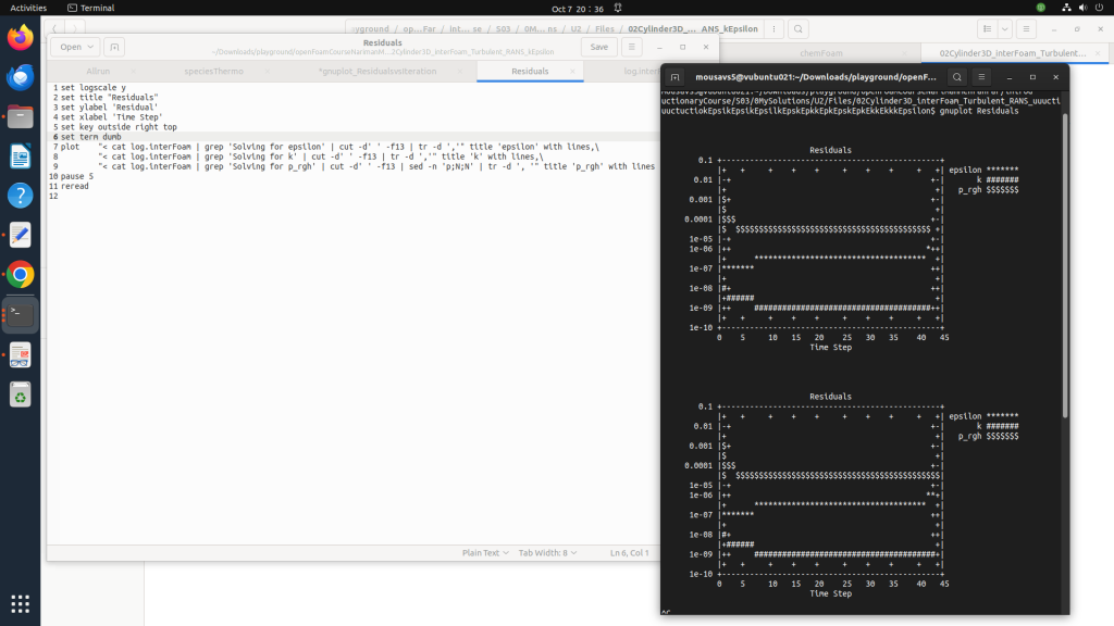
gnuplot Residuals

This will visualize the residuals in real-time, either directly in the terminal (if using SSH) or in the GNUplot GUI, providing a dynamic insight into the convergence of your simulation.

The ‘set term dumb‘ command in GNUplot scripts elegantly bridges the gap between immediate, terminal-based data visualization and the more detailed graphical plotting available in a GUI environment. By transforming numerical data into ASCII art plots directly within the terminal, it provides a swift and straightforward visualization method, especially useful in GUI-less environments like remote servers accessed via SSH. Conversely, omitting or commenting out this command defaults GNUplot to its GUI mode, unlocking a rich, interactive, and detailed visualization experience, thereby catering to varied needs and contexts in data exploration and analysis.

---

Conclusion

Embarking on the journey through the numerical waves of CFD simulations with OpenFOAM and subsequently visualizing the crucial residuals with GNUplot, I’ve navigated through a succinct guide that intertwines the computational prowess of these tools. From extracting pivotal data with a crafted GNUplot script to visualizing it in both terminal and GUI environments, this guide has aimed to illuminate a path for enhanced data analysis and decision-making in your CFD simulations.

The study case, providing a practical application of these steps, can be downloaded using the button below, offering a hands-on experience to further cement your understanding.

Your experiences, insights, and questions are not only welcomed but immensely valued. Engage in the comments section below to share your thoughts or seek clarifications on any step of the process. Whether you’re a seasoned CFD analyst or embarking on your initial simulations, your feedback propels our collective knowledge forward.

Thank you for navigating through this guide with me. May your simulations be stable, and your residuals always converge!